Creating models

What is a model? Why not use solvers directly?

jijmodeling is a “modeler” library which translates human-readable mathematical models into a computer-readable data format. There are several types of optimization problems and corresponding problem-specific solvers which only accept their own specific data format, which in turn require incorporating data specific to a given problem instance. Using jijmodeling, you can write your optimization model in a single and mathematical way, then adapt it to solver and instance-specific details later.

Example model

Let us consider a simple binary linear minimization problem with $N$ real coefficients $d_n$:

$$\min \sum_{n=0}^{N−1}d_n x_n, \\ \text{s.t.} \space \sum_{n=0}^{N-1} x_n = 1, \\ \text{where} \space x_n \in \{0,1\} \space \forall n \in [0, N-1]$$

as an example for demonstrating the basic usage of jijmodeling including

• Define the decision variable $x_n$ and parameters $N$ and $d_n$
• Set the objective function as the minimization of $\sum_{n=0}^{N-1} d_n x_n$
• Add the equality constraint $\sum_{n=0}^{N-1} x_n = 1$

You can find more practical and comprehensive examples on the Learn page.

Create Problem object

Let’s start talking with code. First, we need to import jijmodeling

import jijmodeling as jm
jm.__version__   # 1.0.1

We strongly encourage you to check the version of jijmodeling in your environment is match to this document before trying to run following codes.

The role of Problem is to represent the mathematical model as a Python object.

# Define parameters
d = jm.Placeholder("d", ndim=1)
N = d.len_at(0, latex="N")

# Define decision variables
x = jm.BinaryVar("x", shape=(N,))

# Index for calc sum
n = jm.Element('n', belong_to=(0, N))

# create problem instance 
problem = jm.Problem('my_first_problem')
# Set objective
problem += jm.sum(n, d[n] * x[n])
# Set constraint
problem += jm.Constraint("onehot", jm.sum(n, x[n]) == 1)

# See problem on REPL/Jupyter
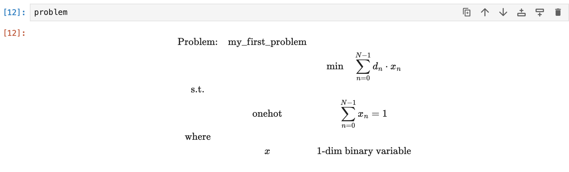
problem

We believe you can find which part of code corresponds to the above mathematical model. This document discusses the concept of each type and their operations a little deeper.

Jupyter Integration

In jupyter or related environment, you can show the contents of a problem object as follows. This will help you to debug your model interactively.

Decision variables and Parameters

There two kinds of "variables" in the above model: Decision variables and parameters. In jijmodeling this is determined by the class used when declaring the object.

• The values of $x_n$ are determined by solving the problem. These are called “decision variables”.
  • In this problem we're using binary variables $x_n \in \{0, 1\}$ represented by BinaryVar. There are other types to choose from to define decision variables, like IntegerVar or ContinuousVar.
  • We'll talk more about the different variable types in Variable types and Bounds.
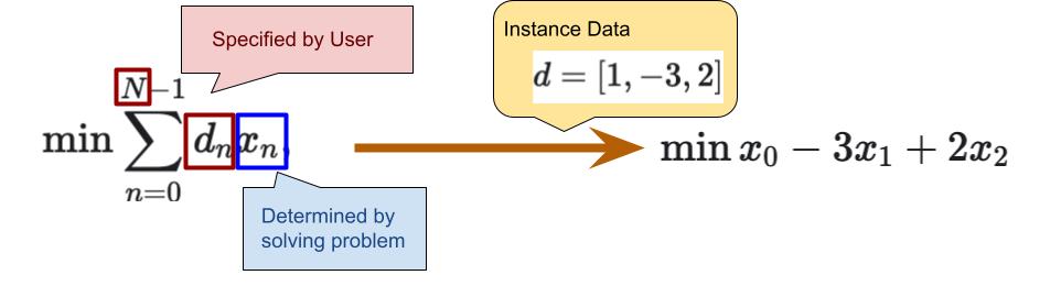
• The values of $N$ and $d$ are "blanks" left to be specified by the user.
  • We say the problem is parametrized by $N$ and $d$.
  • Their actual numerical values are not specified within the Problem object.
  • These can be thought of as part of the "instance data" of the problem. Specific instances will have different values, but we can write the model in a way that is agnostic to those specific values.
  • Most parameters are represented by Placeholder objects defined explicitly, like d in the above code.
  • We defined N as the number of elements in d (it's an ArrayLength object). This makes N an implicit parameter: we only have to specify d to define an instance. This also makes the meaning of $N$ within the mathematical model a clear part of our code.

What is an Object?

In Python, every value has its type. For example, 1 is of type int, and 1.0 is of type float. We can get it by built-in function type like type(1.0). For some type A, we call a value of type A as “A object“.

Multidimensional variables

We can define variables that can be used with indices. This is analogous to having an array or matrix of variables. We want there to be $N$ coefficients $d_n$ and $N$ decision variables $x_n$, so we write them as a one-dimensional Placeholder d and a one-dimensional BinaryVar x. With Placeholders we can just say that it's one-dimensional, without specifying how many values there will be. With decision variables, however, their amount must be specified along with the number of dimensions. But that amount can be defined in relation to parameters, you don't have to use literal numerical value, like so:

# we first define d
d = jm.Placeholder("d", ndim=1)
# and then take the size of it as N
N = d.len_at(0, latex="N")
# x is defined with this size
x = jm.BinaryVar("x", shape=(N,))

The object N is of type ArrayLength, which represents the number of elements in the Placeholder d. The 0 parameter given to len_at is because Placeholders can have any number of dimensions, but for the length to be well-defined we need to specify along the axis we're counting.

info

Indexing and summation will be discussed more deeply in the next page.

Objective function

Next, we want to set $\sum_{n=0}^{N-1} d_n x_n$ as the minimization target of the problem. But $N$ is not fixed yet, and thus we cannot write a for loop in Python. How do we sum up them?

jm.sum exists for resolving this problem:

n = jm.Element('n', belong_to=(0, N))
sum_dx = jm.sum(n, d[n] * x[n])

Element is a new variable type corresponding to indices within some range. In mathematics, we usually consider

For a given $n \in [0, N-1]$, take $n$-th element of $d \in \mathbb{R}^N$.

In jijmodeling that is represented with an Element object n corresponding to $n \in [0, N-1]$ and an expression d[n] corresponding to $d_n$. Be sure that a valid range of indices is stored in Element object. sum takes the element n as its index and expression d[n] * x[n] and returns new expression correspond to $\sum_n d_n x_n$.

info

"Expressions" are discussed deeply in the next page.

Here we can create Problem instance and set $\sum_n d_n x_n$ as the objective function:

problem = jm.Problem('my_first_problem')
problem += sum_dx

If you want to maximize the objective function, you can set the sense parameter when constructing a Problem:

problem = jm.Problem('my_first_problem', sense=jm.ProblemSense.MAXIMIZE)

Equality constraint

Finally, let’s create a Constraint object corresponding to the equality constraint

$$\sum_{n=0}^{N-1} x_n = 1$$

Using sum expression as discussed above, this constraint can be written as an expression:

jm.sum(n, x[n]) == 1

Different from usual Python types whose == return bool value, == for jijmodeling expressions returns a new expression which represents the equality comparison. A Constraint object is created with a name and valid comparison expression (using ==, <= or >=). We can then add it to our problem:

problem += jm.Constraint("onehot", jm.sum(n, x[n]) == 1)

info

This topic will be discussed more deeply in Constraint and Penalty page.