Expressions

What is an expression?

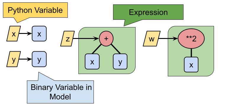
In mathematics, we consider binary or unary operations on integer or real variables, e.g. $x + y$ or $x^2$. Corresponding operations are possible for variables defined in jijmodeling, and their results are called “expressions”:

x = jm.BinaryVar("x")
y = jm.BinaryVar("y")
z = x + y
w = x ** 2

x and y are BinaryVar objects, and z and w are expressions. This is somewhat different from “dependent variables”. z is not a variable in the problem we are considering.

Builtin operators

Python’s built-in operators e.g. + are overloaded for both decision variables (e.g. BinaryVar) and Placeholders:

x = jm.BinaryVar("x")
y = jm.BinaryVar("y")
z = x + y
repr(z)  # "BinaryVar(name='x', shape=[]) + BinaryVar(name='y', shape=[])"

This is a symbolical process, i.e. z is an expression tree like above. We can show the contents of the expression tree by the Python built-in function repr, or we will get more beautiful display using LaTeX if you are in Jupyter environment.

Order of expression

Operator overloading is not limited to linear operations, and we can check an expression only contains linear term using is_linear function:

x = jm.BinaryVar("x")
jm.is_linear(x)  # True
w = x ** 2
jm.is_linear(w)  # False

There are also is_quadratic and is_higher_order to check the order of expressions.

Comparison operators

The equality operator == and other comparison operators e.g. <= are also overloaded to represent equality and inequality constraints. If you want to check if two expression trees are the same, you can use is_same function:

x = jm.BinaryVar("x")
y = jm.BinaryVar("y")
repr(x == y) # "BinaryVar(name='x', shape=[]) == BinaryVar(name='y', shape=[])"
jm.is_same(x, y) # False

Indexing and Summation

Similar to Python’s built-in list or numpy.ndarray, jijmodeling supports indexing to access elements of multidimensional decision variables or parameters:

x = jm.BinaryVar("x", shape=(3, 4))
x[0, 2]

info

x[0][2] and x[0, 2] are equivalent.

x[0, 2] is also an expression. This is similar to the case of x ** 2, which is an expression tree of the unary operator **2 applied to x. x[0] is an expression tree of the "take 0-th element" unary operator [0] applied to x. The subscript can be an expression that contains no decision variables:

x = jm.BinaryVar("x", shape=(3, 4))
n = jm.Placeholder("n")
x[2*n, 3*n]

There is another type of variable for indexing, Element. It is used to represent internal variables like $n$ in

$$\sum_{n=0}^{N-1} x_n .$$

To represent this summation, jijmodeling takes three steps:

N = jm.Placeholder("N")
x = jm.BinaryVar("x", shape=(N,))

# Introduce an internal variable $n$ with its range $[0, N-1]$
n = jm.Element('n', belong_to=(0, N))

# Create operand expression $x_n$ using indexing expression
xn = x[n]

# Sum up integrand expression $x_n$ about the index $n$
jm.sum(n, xn)

$$\mathrm{jm.sum(\overbrace{n}^{subscript}, \underbrace{x[n]}_{operand})}$$

tip

Such a simple sum can be written in abbreviated form as follows

N = jm.Placeholder('N')
x = jm.BinaryVar(name='x', shape=(N,))
sum_x = x[:].sum()

Since the Element object itself can be treated as an expression, we can write $\sum_n n x_n$ as

jm.sum(n, n * x[n])

The result of jm.sum is also an expression. This is helpful for modeling a complicated function repeating same portion like

$$\left(\sum_{n=0}^{N-1} x_n \right) \left(1 - \sum_{n=0}^{N-1} x_n \right)$$

into simple code:

n = jm.Element('n', belong_to=(0, N))
sum_x = jm.sum(n, x[n])
sum_x * (1 - sum_x)

Iterating over a Set

Mathematical models often take the sum over some set $V$, such as

$$\sum_{v \in V} x_v .$$

For example, non-sequential indices like $[1, 4, 5, 9]$ or $[2, 6]$ are used as a set $V$.

tip

Such custom summations often appear in constraint like one-hot constraint for a given index set $V$:

$$\sum_{v \in V} x_v = 1$$

All expressions explained in this page can be used also in Constraint objects.

N = jm.Placeholder('N')
x = jm.BinaryVar('x', shape=(N,))

# `V` is defined as a `Placeholder` object
V = jm.Placeholder('V', ndim=1)

# `V` can be passed as the argument of `belong_to` option
v = jm.Element('v', belong_to=V)

# This `Element` object can be used for summation
sum_v = jm.sum(v, v*x[v])

Actual $V$ is passed as an instance data:

import jijmodeling_transpiler as jmt

problem = jm.Problem('Iterating over a Set')
problem += sum_v

instance_data = { "N": 4, "V": [1, 4, 5, 9]}
compiled_model = jmt.core.compile_model(problem, instance_data)

Jagged array

Sometimes we need to consider a series of index sets $C_\alpha$, for example, to impose K-hot constraints:

$$\sum_{i \in C_\alpha} x_i = K_\alpha.$$

These index sets may be of different lengths, e.g.

$$\begin{align*} C_1 &= [1, 4, 5, 9], \\ C_2 &= [2, 6], \\ C_3 &= [3, 7, 8] \end{align*}$$

Placeholder object can be used to represent such a jagged array:

N = jm.Placeholder('N')
x = jm.BinaryVar('x', shape=(N,))

# Define as 2-dim parameter
C = jm.Placeholder('C', ndim=2)

# Number of K-hot constraints
# Be sure we cannot take `C.len_at(1)` since `C` will be a jagged array
M = C.len_at(0, latex="M")

K = jm.Placeholder('K', ndim=1)

# Usual index
a = jm.Element(name='a', belong_to=(0, M), latex=r"\alpha")
# `belong_to` can take expression, `C[a]`
i = jm.Element(name='i', belong_to=C[a]) 

# K-hot constraint
k_hot = jm.Constraint('k-hot_constraint', jm.sum(i, x[i]) == K[a], forall=a)

Then the actual data is passed as follows:

problem = jm.Problem('K-hot')
problem += k_hot

instance_data = {
    "N": 4,
    "C": [[1, 4, 5, 9],
          [2, 6],
          [3, 7, 8]],
    "K": [1, 1, 2],
}
compiled_model = jmt.core.compile_model(problem, instance_data)

Summation over multiple indices

To compute multiple sums, one may write them in a formula as follows:

$$\sum_{i, j} Q_{ij} x_{ij}$$

This can be implemented in JijModeling as follows.

# set variables
Q = jm.Placeholder('Q', ndim=2)
I = Q.shape[0]
J = Q.shape[1]
x = jm.BinaryVar('x', shape=(I, J))
i = jm.Element(name='i', belong_to=(0, I))
j = jm.Element(name='j', belong_to=(0, J))
# compute the sum over the two indices i, j
sum_ij = jm.sum([i, j], Q[i, j]*x[i, j])

If there are multiple sums, multiple jm.sum can be omitted by making the subscripts a list [subscript1, subscript2, ...]. Of course, this can be written as $\sum_{i, j} = \sum_{i} \sum_{j}$, as can be seen from

sum_ij = jm.sum(i, jm.sum(j, Q[i, j]*x[i, j]))

Conditional Summation

In addition to summing over the entire range of possible indices, you may want to sum only if the indexes satisfy certain conditions, as in the following.

$$\sum_{i<U} x_i$$

This can be implemented using JijModeling as follows

# Define variables to be used
I = jm.Placeholder('I')
x = jm.BinaryVar('x', shape=(I,))
i = jm.Element(name='i', belong_to=(0, I))
U = jm.Placeholder('U')
# Calculate sum only for parts satisfying i<U
sum_i = jm.sum((i, i<U), x[i])

In the part of jm.sum specifying the index, use a tuple to specify (index, condition) like this.

$$\mathrm{jm.sum((\underbrace{i}_{index}, \overbrace{i<U}^{condition}), \underbrace{x[i]}_{operand})}$$

The comparison operators <, <=, >=, >, ==, != and logical operators &, | and their combinations can be used for the conditional expression that the subscript satisfies. For example,

$$\sum_{\substack{i < U \\ i!=N}} d_i x_i$$

can be implemented as follows

# Define variables to be used
d = jm.Placeholder('d', ndim=1)
I = d.shape[0]
x = jm.BinaryVar('x', shape=(I,))
U = jm.Placeholder('U')
N = jm.Placeholder('N')
i = jm.Element(name='i', belong_to=(0, I))
# Calculate sum only for the part satisfying i<U and i≠N
sum_i = jm.sum((i, (i<U)&(i!=N)), d[i]*x[i])

$$\mathrm{jm.sum((\underbrace{i}_{subscript}, \overbrace{(i<U)}^{condition 1} \underbrace{\&}_{logical operator} \overbrace{(i!=N)}^{condition 2}), \underbrace{d[i]*x[i ]}_{operand})}$$

Multiple Summation with Conditions

If there is a condition on the subscripts in a sum operation on multiple subscripts, e.g.

$$\sum_{\substack{i>L \\ i!=N}} \sum_{j<i} R_{ij} x_{ij}$$

A formula such as the following can be implemented as follows

# Define variables to be used
R = jm.Placeholder('R', ndim=2)
I = R.shape[0]
J = R.shape[1]
x = jm.BinaryVar('x', shape=(I, J))
i = jm.Element(name='i', belong_to=(0, I))
j = jm.Element(name='j', belong_to=(0, J))
N = jm.Placeholder('N')
L = jm.Placeholder('L')
# Calculate sum only for the part satisfying i>L and i!=N and j<i
sum_ij = jm.sum([(i, (i>L)&(i!=N)), (j, j<i)], R[i, j]*x[i, j])

The part of jm.sum specifying the indexes should be replaced with [[(index 1, condition of index 1), (index 2, condition of index 2), ...]] By making it look like [(index1, condition of index1), (index2, condition of index2), ...]', multiple sum operations can be written with conditions attached to each index.

caution

[(j, j<i), (i, (i>L)&(i!=N))] will occur an error because $i$ is not yet defined in the $j<i$ part. This can be written in a formula like $\sum_{\substack{i>L \\ i!=N}} \left( \sum_{j<i} \cdots \right)$, but $\sum_{j<i} \left( \sum_{\substack{i>L \\ i!=N}} \cdots \right)$ corresponds to the fact that it cannot be written as Please note the order in which conditions are imposed on subscripts in multiple sums.