JijZeptLab Solver Tutorial
In this tutorial, we will learn how to use JijZeptLab solver. The solver includes:
- MIP solver
- Supports linear programming and mixed integer programming
- NLP solver
- Supports nonlinear programming
Solve with MIP solver
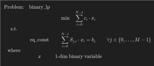
Let us solve the following Binary Linear Programming problem with MIP solver.
import jijmodeling as jm

# set problem
problem = jm.Problem('binary_lp')

# define variables
S = jm.Placeholder('S', ndim=2)
M = S.len_at(0, latex="M")
N = S.len_at(1, latex="N")
b = jm.Placeholder('b', ndim=1)
c = jm.Placeholder('c', ndim=1)
x = jm.BinaryVar('x', shape=(N,))
i = jm.Element('i', belong_to=(0, N))
j = jm.Element('j', belong_to=(0, M))


# Objective
problem += jm.sum(i, c[i]*x[i])

# Constriants
problem += jm.Constraint("eq_const", jm.sum(i, S[j, i] * x[i]) == b[j], forall=j)


# instance data
# set S matrix
inst_S = [[0, 2.3, 0, 2, 0], [1.1, 0, 1, 0, 1], [1, 2, 3, 2, 1]]
# set b vector
inst_b = [2, 2, 6]
# set c vector
inst_c = [1, 2, 3, 4, 5]
instance_data = {'S': inst_S, 'b': inst_b, 'c': inst_c}
Compile the problem
To solve the problem with MIP solver, we need to compile the problem to generate intermediate representation.
import jijzeptlab as jzl

compiled_model = jzl.compile_model(problem, instance_data)
Solve the problem
To solve the problem with MIP solver, we need to do the following steps:
- Create MIP model by using
mip.create_model - Solve the model by using
mip.solve - Convert the result to
jm.SampleSet
import jijzeptlab.solver.mip as mip
mip_model = mip.create_model(compiled_model)
mip_result = mip.solve(mip_model)
print(mip_result.to_sample_set())
The output solution is as follows (jm.SampleSet datatype):
SampleSet(record=Record(solution={'x': [(([2, 3, 4],), [1.0, 1.0, 1.0], (5,))]}, num_occurrences=[1]), evaluation=Evaluation(energy=[], objective=[12.0], constraint_violations={"eq_const": [0.0]}, penalty={}), measuring_time=MeasuringTime(solve=SolvingTime(preprocess=None, solve=None, postprocess=None), system=SystemTime(post_problem_and_instance_data=None, request_queue=None, fetch_problem_and_instance_data=None, fetch_result=None, deserialize_solution=None), total=None), metadata={})
MipModelOption and MipSolveOption
MipModelOption and MipSolveOption allows users to specify the following options:
import jijzeptlab.solver.mip as mip

option = mip.MipModelOption(
    relaxed_variable_names=["x"], # specify relaxed variables to continuous variables
    relax_all_variables=False, # set whether to relax all variables to continuous variables
    solver_name="CBC", # set solver name. Available solvers are "CBC", "GUROBI"
    emphasis="FEASIBILITY", # set solver emphasis. available options are "FEASIBILITY", "OPTIMALITY", and "DEFAULT"
    infeas_tol=1e-4, # set infeasibility tolerance
    integer_tol=1e-4, # set integer tolerance
    max_mip_gap=1e-4, # set maximum MIP gap
    max_mip_gap_abs=1e-4, # set maximum MIP gap (absolute)
)

mip_model = mip.create_model(compiled_model, option=option)

solve_option = mip.MipSolveOption(
    max_seconds=10, # set maximum seconds to solve
    max_nodes=100, # set maximum nodes to solve
    max_solutions=10, # set maximum solutions to solve
    max_seconds_same_incumbent=10, # set maximum seconds to solve with the same incumbent
    max_nodes_same_incumbent=100, # set maximum nodes to solve with the same incumbent
    relax=True, # set whether to relax the problem
)

mip_result = mip.solve(mip_model, solve_option=solve_option)
Solve with NLP solver
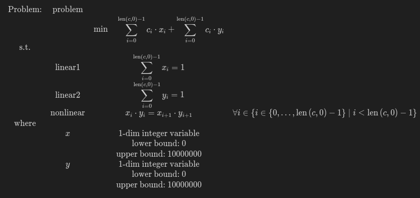
Let us solve the following Nonlinear Programming problem with NLP solver.
import jijmodeling as jm
import jijzeptlab as jzl
import numpy as np

c = jm.Placeholder("c", ndim=1)
x = jm.IntegerVar("x", shape=(c.shape[0],), lower_bound=0, upper_bound=10000000)
y = jm.IntegerVar("y", shape=(c.shape[0],), lower_bound=0, upper_bound=10000000)
i = jm.Element("i", belong_to=c.shape[0])

objective = jm.sum(i, c[i] * x[i]) + jm.sum(i, c[i] * y[i])
problem = jm.Problem("problem")
problem += objective
problem += jm.Constraint("linear1", jm.sum(i, x[i]) == 1)
problem += jm.Constraint("linear2", jm.sum(i, y[i]) == 1)
problem += jm.Constraint(
    "nonlinear",
    x[i] * y[i] == x[i + 1] * y[i + 1],
    forall=[(i, i < c.shape[0] - 1)],
)

instance_data = {"c": np.array([2, 4, 6, 8, 10])}

compiled_model = jzl.compile_model(problem, instance_data)
Solve the problem
Solving the problem with NLP solver is basically the same as MIP solver.
import jijzeptlab.solver.nlp as nlp

nlp_model = nlp.create_model(compiled_model, )
nlp_result = nlp.solve(nlp_model)
print(nlp_result.to_sample_set())
NlpModelOption and NlpSolverOption
NlpModelOption and NlpSolverOption allows users to specify the following options:
model_option = nlp.NlpModelOption(
    relaxed_variable_names=["x", "y"], # specify relaxed variables to continuous variables
    relax_all_variables=False, # set whether to relax all variables to continuous variables
)

solver_option = nlp.NlpSolverOption(
    solver = "ipopt" # set solver name. Available solvers are "ipopt", "gurobi". Note that "ipopt" returns relaxed variable solutions.
)

nlp_model = nlp.create_model(compiled_model, model_option=model_option, solver_option=solver_option)
nlp_result = nlp.solve(nlp_model)
print(nlp_result.to_sample_set())
Solve the QUBO problem
Let us solve the following QUBO problem with SA sampler.
import jijmodeling as jm

# set problem
problem = jm.Problem('QUBO')

# define variables
N = jm.Placeholder('N')
a = jm.Placeholder('a', ndim=2)
x = jm.BinaryVar('x', shape=(N,N))
i = jm.Element('i', belong_to=(0, N))
j = jm.Element('j', belong_to=(0, N))


# Objective
problem += jm.sum([i, j], a[i, j]*x[i, j])

# Constriants
problem += jm.Constraint('onehot-row', x[:, j].sum() == 1, forall=j)
problem += jm.Constraint('onehot-col', x[i, :].sum() == 1, forall=i)


# instance data
instance_data = {
 "N": 3,
 "a": [[1, 2, 3],
       [4, 5, 6],
       [7, 8, 9]]
}
Compile the problem
To solve the problem with SA sampler, we need to compile the problem to generate intermediate representation.
import jijzeptlab as jzl

compiled_model = jzl.compile_model(problem, instance_data)
Solve the problem
- Create SA model by using
sa.create_model - Solve the model by using
sa.sample - Convert the result to
jm.SampleSet
import jijzeptlab.sampler.sa as sa

sa_model = sa.create_model(compiled_model)
sa_result = sa.sample(sa_model)
print(sa_result.to_sample_set())
SampleSet(record=Record(solution={'x': [(([0, 1, 2], [2, 1, 0]), [1.0, 1.0, 1.0], (3, 3))]}, num_occurrences=[1]), evaluation=Evaluation(energy=[-27.0], objective=[15.0], constraint_violations={"onehot-col": [0.0], "onehot-row": [0.0]}, penalty={}), measuring_time=MeasuringTime(solve=SolvingTime(preprocess=None, solve=None, postprocess=None), system=SystemTime(post_problem_and_instance_data=None, request_queue=None, fetch_problem_and_instance_data=None, fetch_result=None, deserialize_solution=None), total=None), metadata={'system': [], 'sampling_time': 1417.6669938024133, 'execution_time': 1284.2910073231906, 'list_exec_times': array([1284.29100732]), 'schedule': {'beta_max': 1.3157629102823118, 'beta_min': 0.027182242374899815, 'num_sweeps': 1000}})
SASamplerOption
SASamplerOption allows users to specify the following options:
import jijzeptlab.sampler.sa as sa

option = sa.SASamplerOption(
    beta_min = 0.1, #set a minimum (initial) inverse temperature
    beta_max = 10, #set a maximum (final) inverse temperature
    num_sweeps = 2000, #set a number of Monte-Carlo steps
    num_reads = 5, #set a number of samples
    initial_state = None, #set a an initial state(dict)
    updater= "swendsen wang", #set an updater algorithm. Available options are "single spin flip" and "swendsen wang"
    sparse = True, #set whether only non-zero matrix elements are stored, which will save memory.
    reinitialize_state = False, #set whether to reinitialize state for each run
    seed = None, #set a seed for Monte Carlo algorithm
)
#specify other options when compling the model
compiled_model.set_default_parameters(multipliers ={"onehot-row": 10, "onehot-col": 10},needs_square_dict={"onehot-rol": False,"onehot-row": False})
sa_model = sa.create_model(compiled_model)
sa_result = sa.sample(sa_model,option=option)
print(sa_result.to_sample_set())