Traveling Salesman Problem with parameter search

The Travelling Salesman Problem (TSP) is a very well-known problem of finding the shortest path between every city. Obviously there are two limitations on this problem: every time the salesman can only be in one city and all the cities have to be visited only once. In this notebook, we only consider a quadratic formulation of TSP due to its annealing properties.

Mathematical model of TSP

The objective function of TSP is the total distance of the path that the salesman goes through.

$$\begin{aligned}\min_x \quad &\sum_{i,j,t}d_{i,j}x_{i,t}x_{j,(t+1)\bmod n} \\ \textrm{s.t.} \quad &\sum_t x_{i,t}=1,\quad \forall i \in \{0,\ldots, n-1\} \\ &\sum_i x_{i,t}=1,\quad \forall t \in \{0,\ldots, n-1\}\end{aligned}$$

where $d_{i,j} \geq 0$, a distance between city $i$ and city $j$.

$x_{i,t}$ is a binary variables such as $x_{i,t} = \begin{cases} 1 & \text{t-th city i} \\ 0 & \text{otherwise} \end{cases}, \qquad \forall i,t\in \{0,\ldots,n-1\}\\$ $x_{i,t}=1$ represents the salesman visits city $i$ at $t$. $\bmod n$ is used to take into account of the distance between the last city and the first city.

Moreover, we have to consider the two constraints mentioned above:

1. Every city can only be visited once, $\sum_t x_{i,t}=1,\quad \forall i$.
2. The salesman can only be one city at a time t, $\sum_i x_{i,t}=1,\quad \forall t$

Penalty term

For a solver like QUBO, it is required to be an unconstrained function. In order to convert a constrained optimization problem such as TSP into an unconstrained one, the constraints can be converted to penalty terms, which is called the Penalty Method. Typically the penalty terms are nothing but squares of the constraints function and contain penalty coefficients or multipliers. The way to find the suitable values in these coefficients is known as "parameter search".

Therefore the final objective function of TSP will be

$\min_x\quad \sum_{i,j,t}d_{i,j}\cdot x_{i,t}\cdot x_{j,(t+1)\bmod n}+ \lambda_1 (\sum_i x_{i,t}-1)^2 + \lambda_2 (\sum_t x_{i,t}-1)^2$

Tuning of the multipliers can help the solver find the optimal feasible solution easily. If the coefficients $\pmb{\lambda}=\{\lambda_1,\lambda_2\}$ is too small or even 0, the objective function will be closed or equal to $\sum_{i,j,t}d_{i,j}\cdot x_{i,t}\cdot x_{j,(t+1)\bmod n}$. The constraint condition will be almost or completely ignored, so that infeasible solutions are yielded. On the other hand, if the multiplier $\pmb{\lambda}$ is too large, the penalty term will dominate, which can be thought of the objective function are closed to $\lambda_1 (\sum_i x_{i,t}-1)^2 + \lambda_2 (\sum_t x_{i,t}-1)^2$. The solver now finds the solutions by emphasising the constraint condition, so that it leads to obtain feasible solutions but not optimal.

Implementing TSP with parameter search in JijZeptLab

Now we are considering how to solve this problem by using JijZeptLab.

import jijmodeling as jm
import numpy as np
import matplotlib.pyplot as plt
import jijzeptlab as jzl
client = jzl.client.JijZeptLabClient(config="./config.toml")

#define a JijModel of TSP
d = jm.Placeholder("d", ndim=2)
n = d.len_at(0, latex="n")
i, j, t = jm.Element("i", n), jm.Element("j", n), jm.Element("t", n)

# binary variable
x = jm.BinaryVar("x", shape=(n, n))

problem = jm.Problem("TSP")
# Objective function
problem += jm.sum([i, j], d[i, j]*jm.sum(t, x[i, t]*x[j, (t+1) % n]))

# Constraints
jmC = jm.Constraint
problem += jmC("one-time", x[i, :].sum() == 1, forall=i)
problem += jmC("one-city", x[:, t].sum() == 1, forall=t)

problem

$\begin{array}{cccc}\text{Problem:} & \text{TSP} & & \\& & \min \quad \displaystyle \sum_{i = 0}^{n - 1} \sum_{j = 0}^{n - 1} d_{i, j} \cdot \sum_{t = 0}^{n - 1} x_{i, t} \cdot x_{j, \left(t + 1\right) \bmod n} & \\\text{{s.t.}} & & & \\ & \text{one-city} & \displaystyle \sum_{\ast_{0} = 0}^{n - 1} x_{\ast_{0}, t} = 1 & \forall t \in \left\{0,\ldots,n - 1\right\} \\ & \text{one-time} & \displaystyle \sum_{\ast_{1} = 0}^{n - 1} x_{i, \ast_{1}} = 1 & \forall i \in \left\{0,\ldots,n - 1\right\} \\\text{{where}} & & & \\& x & 2\text{-dim binary variable}\\\end{array}$

Let's generate points randomly, and one point represents as one city.

def random_2d_tsp(n: int):
    x = np.random.uniform(0, 1, n)
    y = np.random.uniform(0, 1, n)
    #calculate the distances between different points
    XX, YY = np.meshgrid(x, y)
    distance = np.sqrt((XX - XX.T)**2 + (YY - YY.T)**2)
    return distance, (x, y)

#number of city
num_city = 10
# create an instance
distance, (pos_x, pos_y) = random_2d_tsp(n=num_city)
instance_data = {'d': distance}

plt.scatter(pos_x, pos_y)
plt.xlim(0, 1)
plt.ylim(0, 1)
plt.show()

Next we define the script to solve the TSP as a script named "script_on_server_side". Since it is critical to set the penalty term as the distance term (1st term), the strategy of updating the parameter A depends on two scenarios, "no any feasible solutions" or "at least one feasible solution".

First, let's consider the scenario of "no any feasible solutions". The total number of constraint violations is set as the parameter A, and the SA solver is called again. However, if there is still no feasible solution, then it will be solved again with the new parameter, $A \to 2A$ until a feasible solution is found.

Otherwise, the parameter A is needed to adjust as small as possible without violating the constraint conditions. If violation appears, e.g. city $i$ is missing at time $t$, $x_{i,t}=0$, the total number of constraint violations is 2 and a lower value in total distance will certainly be yielded. The maximum decrement in the objective function is $$ di=d{i-1,i}+d{i,i+1}$$, where $d{i-1,i}$ and $d_{i-1,i}$ are missing paths from $(i-1)$ to $i$ and from $i$ to $(i+1)$. Therefore, in order to fulfill the constraint conditions, the parameter has to be adjusted as

$2A > \max \, d_i, \quad \forall i.$

Now, the penalty outweighs the maximum decrement.

Finally introducing a hyper-parameter $\alpha >1 $ is just to act as "greater-than" sign, so that the parameter is

$A = \frac{\alpha}{2} \max \ d_i, \quad \forall i.$

We can use set_default_parameters when compiling the model to set the desired values in the parameters.

The objective function finally becomes

$\min_x\quad \sum_{i=0}^{n-1}\sum_{j=0}^{n-1}d_{i,j}\cdot \sum_{t=0}^{n-1}x_{i,t}\cdot x_{j,(t+1)\bmod n}+ A (\sum_{i=0}^{n-1}x_{i,t}-1)^2 + A (\sum_{t=0}^{n-1}x_{i,t}-1)^2$

The flow chart of the parameter search is below

def script_on_server_side():
    import jijzeptlab as jzl
    import jijmodeling as jm
    import numpy as np
    import jijzeptlab.sampler.sa as sa
    
    # problem, instance_data are pre-defined (passed from client-side)
    problem: jm.Problem
    instance_data: dict
    
    # translate to an array of tour
    def convert_to_tour(nonzero_indices, num_city):
        tour = np.zeros(num_city, dtype=int)
        i_value, t_value = nonzero_indices
        tour[t_value] = i_value
        #connect the last city to the first city 
        tour = np.append(tour, [tour[0]])
        return tour
    
    # no. of updatings
    num_iter = 10
    # no. of trails per updating
    num_reads = 5
    alpha = 1.2
    results = []
    # distance  matrix
    distance = np.array(instance_data['d'])
    num_city = len(distance)
    # Sub. the largest city distance into the multiplier A
    A = np.max(distance)
    Ahistory = [A]
    best_tour = None
    
    best_objective = np.inf
    # compile the problem to generate intermediate representation
    compiled_model = jzl.compile_model(problem, instance_data)
    for i in range(num_iter):
        # re-put the parameters of TSP
        compiled_model.set_default_parameters(multipliers ={"one-city": A, "one-time": A})
        # set the num_reads
        Option = sa.SASamplerOption(num_reads= num_reads)
        # make sa instance
        sa_model = sa.create_model(compiled_model)
        # solve
        sa_result = sa.sample(sa_model,Option)
        # convert the solution to `jm.SampleSet`
        final_solution = sa_result.to_sample_set()
        # obtain feasible solutions
        feasibles = final_solution.feasible()
        if len(feasibles.evaluation.objective) == 0:
            # If no feasible solution is obtained, increase the value of multiplier and try again.
            one_time_violaiton = np.mean(final_solution.evaluation.constraint_violations["one-time"])
            one_city_violaiton = np.mean(final_solution.evaluation.constraint_violations["one-city"])
            A += one_city_violaiton + one_time_violaiton
        else:
            # find the solution with the lowest objective value
            argmin_e = np.argmin(feasibles.evaluation.objective)
            nonzero_indices, _, _ = feasibles.record.solution["x"][argmin_e]
            # convert to an array of the optimal tour
            tour = convert_to_tour(nonzero_indices, num_city)

            # save the best tour
            if feasibles.evaluation.objective[argmin_e] < best_objective:
                best_objective = feasibles.evaluation.objective[argmin_e]
                best_tour = tour
            # construct the array d_i for the updating later
            dij_dik = []
            for t, _i in enumerate(tour):
                _j = tour[(t-1)%num_city]
                _dij = distance[_i, _j]
                _k = tour[(t+1)%num_city]
                _dik = distance[_i, _k]
                dij_dik.append(_dij + _dik)
                
            # Update the value of multiplier
            A = alpha * np.max(dij_dik)/2

        Ahistory.append(A)
        results.append(final_solution)
        

# sent the problem with data to JijZeptLab server and get the result
input_data = jzl.client.InputData(problem, instance_data)
result = client.submit_func(script_on_server_side, ["results","Ahistory"], input_data)

Make a plot with objective and parameter values

# A list of the solutions with different values of multiplier 
sampleset = result.variables['results']
# A list of different values of multiplier  
Ahistory = result.variables['Ahistory']
objective = [np.mean(r.evaluation.objective) for r in sampleset]
fig = plt.figure()

ax1 = fig.add_subplot(111)

ln1 = ax1.plot(Ahistory[:-1], "--", label="A")

ax2 = ax1.twinx()
ln2 = ax2.plot(objective, c="r", label="Objective")


h1, l1 = ax1.get_legend_handles_labels()
h2, l2 = ax2.get_legend_handles_labels()
ax1.legend(h1+h2, l1+l2, loc='upper right', fontsize=15)

ax1.set_xlabel('Step', fontsize=15)
ax1.set_ylabel(r'$A$', fontsize=15)
ax2.set_ylabel('Objective', fontsize=15)

Text(0, 0.5, 'Objective')

The red line represents the average objective values with the same parameter value, which is represented by the blue dot line, at every step. One can see that large parameter value causes large objective value. This can be interpreted as that the optimal process focuses more on the constraint terms, but not enough to optimize the distances between cities.

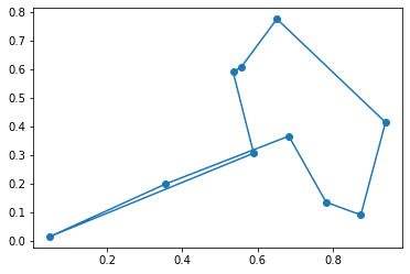
Draw the best tour

# translate to an array of tour
def convert_to_tour(nonzero_indices, num_city):
        tour = np.zeros(num_city, dtype=int)
        i_value, t_value = nonzero_indices
        tour[t_value] = i_value
        tour = np.append(tour, [tour[0]])
        return tour

#get feasible solutions
feasibles = [r.feasible()  for r in sampleset]
#get the average objective values of all the feasible solutions 
objective = [np.mean(r.evaluation.objective) for r in feasibles]
#find the optimal parameter value
argmin_para = np.nanargmin(objective)
#find the lowest objective values 
argmin_e = np.argmin(feasibles[argmin_para].evaluation.objective)
nonzero_indices, _, _ = feasibles[argmin_para].record.solution["x"][argmin_e]

best_tour = convert_to_tour(nonzero_indices, num_city)

/Users/blues/miniforge3/envs/tensorflow/lib/python3.9/site-packages/numpy/core/fromnumeric.py:3464: RuntimeWarning: Mean of empty slice.
  return _methods._mean(a, axis=axis, dtype=dtype,
/Users/blues/miniforge3/envs/tensorflow/lib/python3.9/site-packages/numpy/core/_methods.py:192: RuntimeWarning: invalid value encountered in scalar divide
  ret = ret.dtype.type(ret / rcount)

plt.scatter(pos_x, pos_y)
plt.plot(pos_x[best_tour], pos_y[best_tour], "-")
plt.show()